Metro Network Structure Learning

Objective

This article puts Graph Structure Learning (GSL) into practice on a synthetic subway network. A simple GSL architecture is trained to predict traffic, and the graph it learns is compared to the actual subway network.

The experiment also tests one of GSL’s key promises: resilience, both to noisy data and to a corrupted initial graph.

Data

Data combines two elements:

• A network: a synthetic subway line network.
• A process on that network: synthetic passenger traffic.

Subway network

The metro network is built from a manual configuration specifying each line and its intersections with the others.

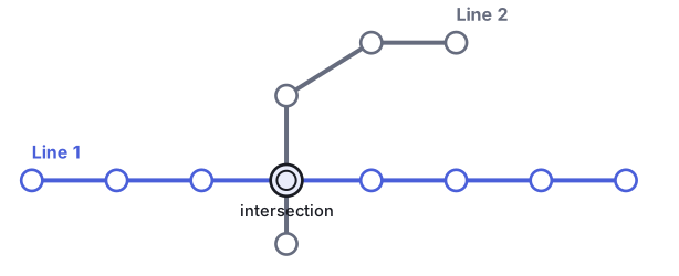
Each station is instantiated as several nodes: one per line, per direction, plus an extra node at intersections. This finer-grained representation should make the traffic pattern easier for the model to learn than a single node per station would.

For readability, the visualizations below aggregate results back to one node per station where possible.

Markov process

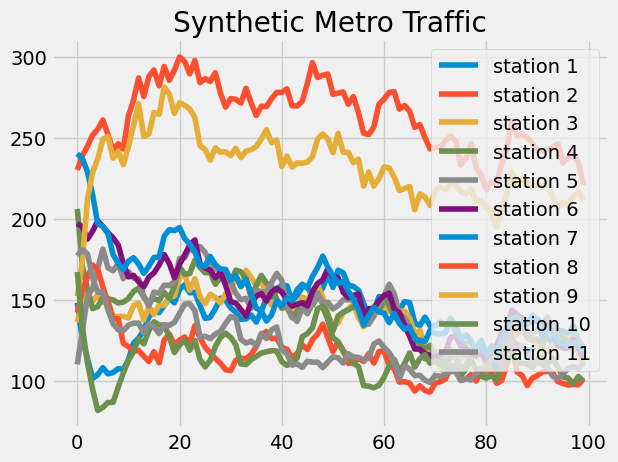
Traffic is generated synthetically as well. Each node starts with a random number of people, then the signal propagates through the network step by step following a Markov process.

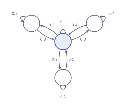
Two parameters control the uncertainty of the data: additive noise and multiplicative noise.

Prediction task

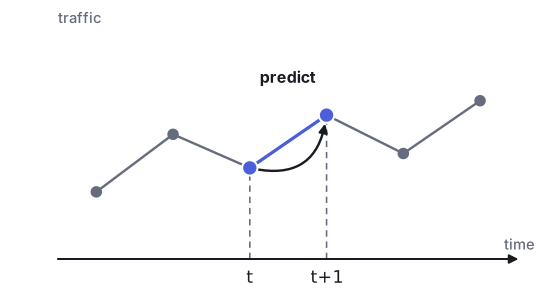
The model described below is auto-regressive: it predicts traffic from previous traffic values, using a single past step to predict the next one. Given how simple the underlying data model is, this single step is enough for accurate prediction.

Model

Graph Structure Learning module

Direct optimization

The adjacency matrix $A$ is optimized directly as a free parameter, defined and initialized in PyTorch as:

self.matrix = nn.Parameter(torch.empty(self.num_nodes, self.num_nodes), requires_grad=True)
torch.nn.init.kaiming_uniform_(self.matrix, a=2.23)

Embedding

Alternatively, each node gets a learned embedding; a distance between embeddings then gives the adjacency matrix:

self.node_embeddings_start = torch.nn.Embedding(num_nodes, embedding_size, sparse=False)
self.node_embeddings_target = torch.nn.Embedding(num_nodes, embedding_size, sparse=False)

Two embeddings are learned per node, so $A_{ij}$ can differ from $A_{ji}$.

Positivity constraint enforcement

Edge weights represent flows of people between stations, so they must stay non-negative. This is enforced architecturally, either with ReLU or an exponential:

# Using exponential function
A = A.exp()
# Using ReLU
A = torch.nn.functional.relu(A)

Sparsity constraint enforcement

Real graphs are sparse, so each node keeps only its top-k neighbors. This is a safe way to enforce sparsity, but it limits the graph’s flexibility and introduces a new hyperparameter k:

values, indices = A.topk(k=self.neighbor_nb+1, dim=dim)
mask = torch.zeros_like(A)
mask.scatter_(dim, indices, values.fill_(1))
A*mask

Alternatives

Simpler alternatives exist for a problem this constrained, and could match or beat this architecture’s performance in less time.

Markov model

Since the data follows a Markov process, a Markov model (MM/HMM) is the obvious baseline. It becomes less relevant once the horizon grows: if traffic at $t$ depends on several past steps $t-1, ..., t-n$ rather than just $t-1$, a Markov model no longer captures it.

Experiments

Construction of the graph

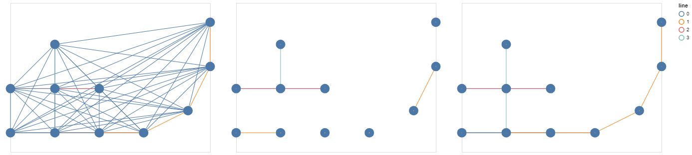
This experiment tracks how the learned graph evolves as the network trains.

The two graphs are compared with two metrics: recall and precision.

$$\text{recall} = \frac{\text{Nb edges correctly learned}}{\text{Total nb reference edges}}$$ $$\text{precision} = \frac{\text{Nb edges correctly learned}}{\text{Total nb learned edges}}$$

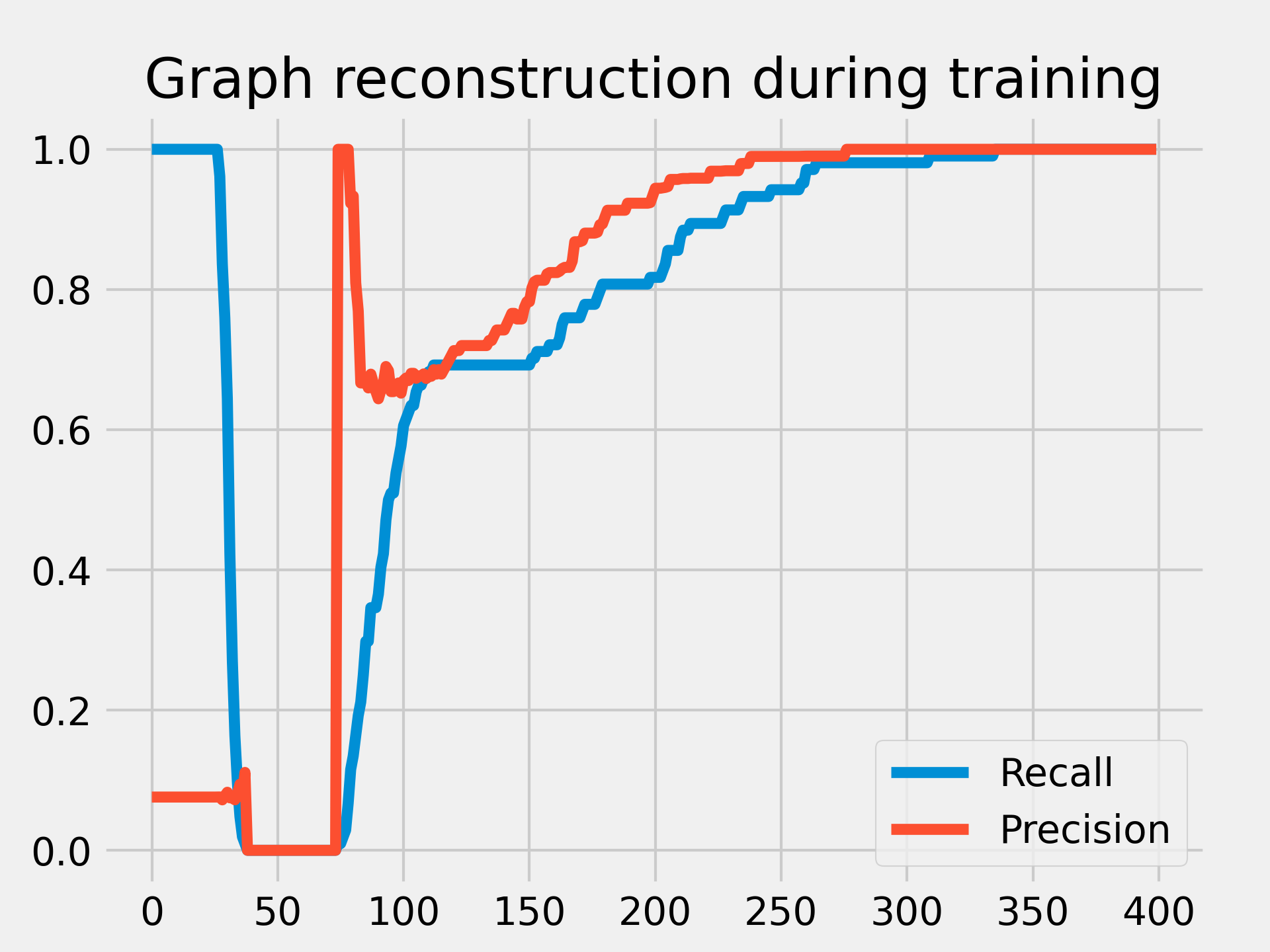
At initialization, the graph is quasi-complete — every pair of nodes is connected, a side effect of the kaiming_uniform initialization. To satisfy the sparsity constraint, it then collapses to fully disconnected, before the model gradually learns the right balance and recovers the exact graph. These phases are visible in the illustration above.

This balance is easy to find in such a simple case. In practice, the graph is rarely recovered exactly.

Noisy data

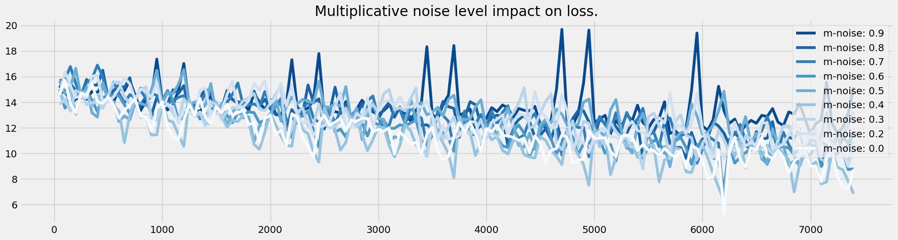
This experiment manipulates the multiplicative and additive noise hyperparameters, to study their impact on both prediction performance and graph retrieval.

Multiplicative noise

The multiplicative noise level is varied between 0 and 1 in steps of 0.1, applied at each step of the signal simulation as:

$$A' = A * (1 + m)$$

with $m \in R^n$ and

$$m_i \sim U\left(-\frac{\text{level}}{2}, \frac{\text{level}}{2}\right)$$

Learning is affected by noise, but the model still converges.

Additive noise

Additive noise follows the same pattern:

$$A' = A + a$$

with $a \in R^n$ and

$$a_i \sim U\left(-\frac{\text{level}}{2}, \frac{\text{level}}{2}\right)$$

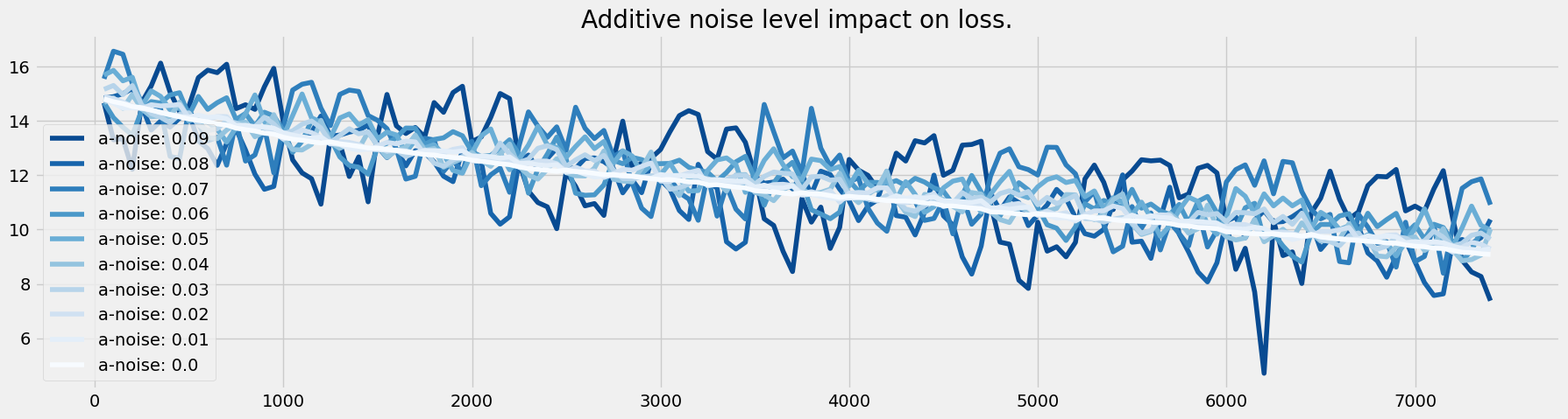
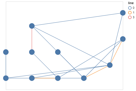
The graph is also recovered despite the noise. At an additive noise level of 0.1, the graph under construction already shows the beginning of the reference network’s structure.

Conclusion

For a case this simple, the GSL module delivers on what is expected of it:

• Reconstruction — it recovers the real network behind the learned signal.
• Resilience to noise — it still learns the correct network from a noisy signal.
• Resilience to initialization — it recovers the original network even from a corrupted starting graph.

This explainability comes with a caveat: it tends to decrease as model capacity grows. MTGNN, for instance, predicts well without producing a graph that is easy to interpret.

Robustness to adversarial attacks on higher-capacity models remains an active research question.

References

Chen, Y., & Wu, L. (2022). Graph Structure Learning. In Graph Neural Networks: Foundations, Frontiers, and Applications (Chapter 14). Springer. https://doi.org/10.1007/978-981-16-6054-2_14

Zhu, Y., Xu, W., Zhang, J., Du, Y., Zhang, J., Liu, Q., Yang, C., & Wu, S. (2021). A Survey on Graph Structure Learning: Progress and Opportunities (arXiv:2103.03036). arXiv. https://doi.org/10.48550/arXiv.2103.03036

Wu, Z., Pan, S., Long, G., Jiang, J., Chang, X., & Zhang, C. (2020). Connecting the Dots: Multivariate Time Series Forecasting with Graph Neural Networks. Proceedings of the 26th ACM SIGKDD International Conference on Knowledge Discovery & Data Mining, 753‑763. https://doi.org/10.1145/3394486.3403118